18.1 GNUPLOT: Display of Functions and Surfaces

Graphical display of functions and data is done via an interface, the REDUCE GNUPLOT¹ package, to the popular gnuplot² graphing utility. It allows you to display functions in 2D and surfaces in 3D on a variety of output devices including X terminals, PC monitors, and postscript and LATEX printer files.

The binary distribution of REDUCE for Microsoft Windows includes gnuplot version 5.4, which has its own documentation. Web REDUCE also includes gnuplot version 5.4. On other platforms, REDUCE uses whatever version of gnuplot is available.

The GNUPLOT package provides easy to use graphics output for curves or surfaces which are defined by formulas and/or data sets, and supports a variety of output devices such as VGA screen, postscript, picTEX, MS Windows. It lets you generate gnuplot graphical output directly from inside REDUCE, either for the interactive display of curves/surfaces or for the production of pictures on paper.

18.1.1 Command plot

Under the REDUCE GNUPLOT package, gnuplot is used as a graphical output server, invoked by the command plot(…). This command can have a variable number of parameters:

• A function to plot, which can be

  • an expression with one unknown, e.g., u*sin(u)^2;

  • a list of expressions with one (identical) unknown, e.g., {sin(u), cos(u)};

  • an expression with two unknowns, e.g., u*sin(u)^2+sqrt(v);

  • a list of expressions with two (identical) unknowns, e.g., {x^2+y^2,x^2-y^2};

  • a parametic expression of the form point(<u>,<v>) (for 2D plots) or point(<u>,<v>,<w>) (for 3D plots) where <u>,<v>,<w> are expressions which depend of one or two parameters; if there is one parameter, the object describes a curve in the plane (only <u> and <v>) or in 3D space; if there are two parameters, the object describes a surface in 3D. The parameters are treated as independent variables. Example: point(sin t,cos t,t/10);

  • an equation with a symbol on the left-hand side and an expression with one or two unknowns on the right-hand side, e.g., dome= 1/(x^2+y^2);

  • an equation with an expression on the left-hand side and a zero on the right-hand side describing implicitly a one-dimensional variety in the plane (implicitly given curve), e.g., x^3 + x*y^2 - 9x = 0, or a two-dimensional surface in three-dimensional Euclidean space;

  • an equation with an expression in two variables on the left-hand side and a list of numbers on the right-hand side; the contour lines corresponding to the given values are drawn, e.g.,
    x^3 - y^2 + x*y = {-2,-1,0,1,2};

  • a list of points in 2 or 3 dimensions, e.g., {{0,0},{0,1},{1,1}} representing a curve;

  • a list of lists of points in 2 or 3 dimensions, e.g.,
    {{{0,0},{0,1},{1,1}}, {{0,0},{0,1},{1,1}}}
    representing a family of curves.

• A range for a variable: this has the form <variable>=(<lower_bound> .. <upper_bound>) where <lower_bound> and <upper_bound> must be expressions which evaluate to numbers. If no range is specified the default range for independent variables is (-10 .. 10) and for the dependent variable it is set to the maximum for the gnuplot executable (using double floats on most IEEE machines). However, each of the variables plot_xrange, plot_yrange, plot_zrange can be assigned an interval of the form (<lower_bound> .. <upper_bound>) that sets the default range for the \(x\), \(y\), \(z\) direction. The \(z\) direction corresponds to the function values or surface height and setting a \(z\)-range flattens the graph at the range limits, which is especially useful for functions with singularities.

  Additionally, the number of interval subdivisions can be assigned as a formal quotient of the form

  <variable>=(<lower_bound> .. <upper_bound>)/<it>

  where <it> is a positive integer; e.g. (1 .. 5)/30 means the interval from 1 to 5 subdivided into 30 pieces of equal size. A subdivision parameter overrides the value of the option points for this variable.

• A plot option, either as a fixed keyword, e.g., hidden3d or as an equation e.g., term=pictex; free text such as titles and labels should be enclosed in string quotes. Further details are given below.

Please note that a space has to be inserted between a number and a dot when specifying an interval, otherwise the REDUCE translator will be misled.

If a function is given as an equation, the left-hand side is mainly used as a label for the axis of the dependent variable.

In two dimensions, plot can be called with more than one explicit function; all curves are drawn in one picture. However, all these must use the same independent variable name. One of the functions can be a point set or a point set list. Normally all functions and point sets are plotted by lines. A point set is drawn by points only if functions and the point set are drawn in one picture.

The same applies to three dimensions with explicit functions. However, an implicitly given curve must be the sole object for one picture.

In 2D implicit and contour plots, as well as 3D surface plots, the ordering of the two independent variables is by default the standard REDUCE ordering, e.g. \(x\), \(y\) rather than \(y\), \(x\). However, if both independent variables are specified explicitly via options of the form <variable> = <range> then the option ordering is used as the variable ordering. In 2D, the first variable is plotted horizontally and the second vertically, and in 3D the first and second independent variables and the dependent variable form a right-handed coordinate system. (See the examples at the end of this section.)

The functional expressions are evaluated in rounded mode. This is done automatically, it is not necessary to turn on rounded mode explicitly.

Examples:

plot(cos x);
plot(s=sin phi, phi=(-3 .. 3));
plot(sin phi, cos phi, phi=(-3 .. 3));
plot (cos sqrt(x^2 + y^2), x=(-3 .. 3), y=(-3 .. 3),
      hidden3d);
plot {{0,0},{0,1},{1,1},{0,0},{1,0},{0,1},
      {0.5,1.5},{1,1},{1,0}};

% parametric: screw

on rounded;
w := for j := 1:200 collect
                {1/j*sin j, 1/j*cos j, j/200}$
plot w;

% parametric: globe
dd := pi/15$
w := for u := dd step dd until pi-dd collect
    for v := 0 step dd until 2pi collect
      {sin(u)*cos(v), sin(u)*sin(v), cos(u)}$
plot w;

% implicit: superposition of polynomials
plot((x^2+y^2-9)*x*y = 0);

Piecewise-defined functions

A composed graph can be defined by a rule-based operator. In that case each rule must contain a clause which restricts the rule application to numeric arguments, e.g.,

   operator my_step1;
   let {my_step1(~x) => -1 when numberp x and x<-pi/2,
        my_step1(~x) =>  1 when numberp x and x>pi/2,
        my_step1(~x) => sin x
            when numberp x and -pi/2<=x and x<=pi/2};
   plot(my_step1(x));

Of course, such a rule may call a procedure:

   procedure my_step3(x);
      if x<-1 then -1 else if x>1 then 1 else x;
   operator my_step2;
   let my_step2(~x) => my_step3(x) when numberp x;
   plot(my_step2(x));

The direct use of a procedure with a numeric if clause is impossible.

Plot options

The following options are specific to the REDUCE plot command:

• points=<integer>: the number of unconditionally computed data points; for a grid, points^2 grid points are used. The default value is 20. The value of points is used only for variables for which no individual interval subdivision has been included in the range specification.

• refine=<integer>: the maximum depth of adaptive interval intersections for 2D plots (only). The default is 8. A value of 0 switches any refinement off. Note that a high value may increase the computing time significantly.

Additional options

Additional gnuplot options are supported via the following syntax in the plot command.

The following options are implemented using the gnuplotset (or unset if the option begins with no) command, which offers far more control than is currently exposed via this interface. Note that the gnuplotreset command, which clears the effect of most set commands (not set term or set output) from previous calls of plot, is always issued before any set commands. See Commands / Set-show and Commands / Reset in the gnuplot documentation or the gnuplot Help for details.

• title=<string>: the specified title is put at the top of the picture.

• xlabel=<string>, ylabel=<string>, and zlabel=<string> for surfaces: the specified axis labels are displayed. If omitted the axes are labeled by the independent and dependent variable names from the expression. Note that xlabel, ylabel, and zlabel here are used in the usual sense, \(x\) for the horizontal and \(y\) for the vertical axis in 2D, and \(z\) for the perpendicular axis in 3D – these names do not refer to the variable names used in the expressions.

       plot(1,x,(4*x^2-1)/2,(x*(12*x^2-5))/3, x=(-1 .. 1),
          ylabel="L(x,n)", title="Legendre Polynomials");
  

• terminal=name: prepare output for device type name. Every installation uses a default terminal as output device; some installations support additional devices such as printers; consult the gnuplot documentation or the gnuplot Help for details.

• output="filename": redirect the output to a file.

• size=<string>: set the size of the plot via the gnuplot command set size <string>, for example…

  • size="s_x,s_y": rescale the graph (not the window) where \(s_x\) and \(s_y\) are scaling factors for the \(x\)- and \(y\)-sizes, e.g.

              plot(1/(x^2+y^2), x=(0.1 .. 5), y=(0.1 .. 5),
                 size="0.7,1");
    

    Defaults are \(s_x=1,s_y=1\). Note that scaling factors greater than 1 will often cause the picture to be too big for the window.

  • size="ratio -1": set the scales so that the unit has the same length on both the \(x\) and \(y\) axes, which is essential for geometrical plots to look correct, e.g.

              plot(x^2+y^2-1=0, x=(-2 .. 2), y=(-2 .. 2),
                 size="ratio -1");
    

• view="r_x,r_z": set the viewpoint in 3 dimensions by turning the object around the \(x\) or \(z\) axis; the values are degrees (integers). Defaults are \(r_x=60,r_z=30\).

       plot(1/(x^2+y^2), x=(0.1 .. 5), y=(0.1 .. 5),
          view="30,130");
  

• logscale: set all axes to use logarithmic scales.

• contour resp. nocontour: in 3 dimensions an additional contour map is drawn (default: nocontour). Note that contour is an option which is executed by gnuplot by interpolating the precomputed function values. If you want to draw contour lines of a delicate formula, you had better use the contour form of the REDUCE plot command as described above.

• surface resp. nosurface: in 3 dimensions the surface is drawn, resp. suppressed (default: surface).

• hidden3d: apply hidden line removal in 3 dimensions.

• pm3d: draw a solid coloured (palette-mapped 3d) surface in 3 dimensions.

The following option is implemented using the gnuplot command with <style>, which offers far more control than is currently exposed via this interface. See Plotting styles in the gnuplot documentation or the gnuplot Help for details.

• style= one of lines, points, linespoints, impulses, dots, errorbars, boxes, boxerrorbars, boxxyerrorbars, candlesticks, financebars, fsteps, histeps, steps, vector, xerrorbars, xyerrorbars, yerrorbars: set the display style.

18.1.2 Paper output

The following example works for a PostScript printer. If your printer uses a different communication, please find the correct setting for the terminal variable in the gnuplot documentation.

For a PostScript output, you need to add the options terminal=postscript and output="filename" to your plot command, e.g.,

plot(sin x, x=(0 .. 10), terminal=postscript,
     output="sin.ps");

18.1.3 Mesh generation for implicit curves

The basic mesh for finding an implicitly-given curve, the \(x,y\) plane is subdivided into an initial set of triangles. Those triangles which have an explicit zero point or which have two points with different signs are refined by subdivision. A further refinement is performed for triangles which do not have exactly two zero neighbours because such places may represent crossings, bifurcations, turning points or other difficulties. The initial subdivision and the refinements are controlled by the option points which is initially set to 20: the initial grid is refined unconditionally until approximately points * points equally-distributed points in the \(x,y\) plane have been generated.

The final mesh can be visualized in the picture by setting

    on show_grid;

18.1.4 Mesh generation for surfaces

By default the functions are computed at predefined mesh points: the ranges are divided by the number associated with the option points in both directions.

For two dimensions the given mesh is adaptively smoothed when the curves are too coarse, especially if singularities are present. On the other hand refinement can be rather time-consuming if used with complicated expressions. You can control it with the option refine. At singularities the graph is interrupted.

In three dimensions no refinement is possible as gnuplot supports surfaces only with a fixed regular grid. In the case of a singularity the near neighborhood is tested; if a point there allows a function evaluation, its clipped value is used instead, otherwise a zero is inserted.

When plotting surfaces in three dimensions you have the option of hidden line removal. Because of an error in Gnuplot 3.2 the axes cannot be labeled correctly when hidden3d is used ; therefore they aren’t labelled at all. Hidden line removal is not available with point lists.

18.1.5 gnuplot operation

The command plotreset; deletes the current gnuplot output window. The next call to plot will then open a new one.

If gnuplot is invoked directly by an output pipe (UNIX and Windows), an eventual error in the gnuplot data transmission might cause gnuplot to quit. As REDUCE is unable to detect the broken pipe, you have to reset the plot system by calling the command plotreset; explicitly. Afterwards new graphics output can be produced.

Under Windows 3.1 and Windows NT, gnuplot has a text and a graph window. If you don’t want to see the text window, iconify it and activate the option update wgnuplot.ini from the graph window system menu – then the present screen layout (including the graph window size) will be saved and the text windows will come up iconified in future. You can also select some more features there and so tailor the graphic output. Before you terminate REDUCE you should terminate the graphic window by calling plotreset;. If you terminate REDUCE without deleting the gnuplot windows, use the command button from the gnuplot text window – it offers an exit function.

18.1.6 Saving gnuplot command sequences

If you want to use the internal gnuplot command sequence more than once (e.g., for producing a picture for a publication), you may set

on trplot, plotkeep;

trplot causes all gnuplot commands to be written additionally to the actual REDUCE output. Normally the data files are erased after calling gnuplot, however with plotkeep on the files are not erased.

18.1.7 Direct Call of gnuplot

gnuplot has a lot of facilities which are not accessed by the operators and parameters described above. Therefore genuine gnuplot commands can be sent by REDUCE. Please consult the gnuplot manual for the available commands and parameters. The general syntax for a gnuplot call inside REDUCE is

    gnuplot(<cmd>,<p_1>,<p_2> ...)

where cmd is a command name and \(p_1,p_2, \ldots \) are the parameters, inside REDUCE separated by commas. The parameters are evaluated by REDUCE and then transmitted to gnuplot in gnuplot syntax. Usually a drawing is built by a sequence of commands which are buffered by REDUCE or the operating system. For terminating and activating them use the REDUCE command plotshow. Example:

     gnuplot(set,polar);
     gnuplot(unset,parametric);
     gnuplot(set,dummy,x);
     gnuplot(plot, x*sin x);
     plotshow;

In this example the function expression is transferred literally to gnuplot, while REDUCE is responsible for computing the function values when plot is called. Note that gnuplot restrictions with respect to variable and function names have to be taken into account when using this type of operation. Important: String quotes are not transferred to the gnuplot executable; if the gnuplot syntax needs string quotes, you must add doubled stringquotes inside the argument string, e.g.,

     gnuplot(plot, """mydata""", "using 2:1");

18.1.8 Examples

The following are taken from a collection of sample plots (gnuplot.tst) and a set of tests for plotting special functions. The pictures are made using the qt gnuplot device and using the menu of the graphics window to export to PDF or PNG.

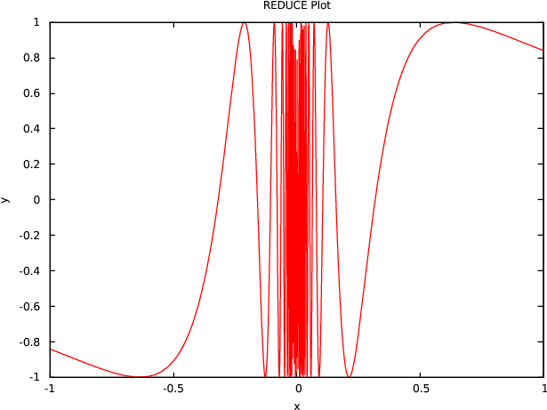
A simple plot for \(\sin (1/x)\):

plot(sin(1/x), x=(-1 .. 1), y=(-3 .. 3));

Some implicitly-defined curves:

plot(x^3 + y^3 - 3*x*y = {0,1,2,3},
     y=(-5 .. 5), x=(-2.5 .. 2));

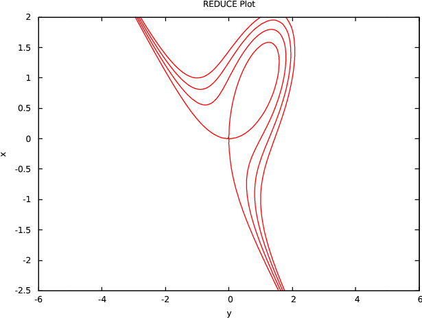
(Note that the \(y\)-axis is plotted horizontally since it is specified first among the options.)

A test for hidden surfaces:

plot(cos sqrt(x^2 + y^2), y=(-3 .. 3), x=(-3 .. 3),
     hidden3d);

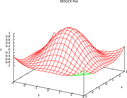
(Note the left-handed coordinate system since \(y\) is specified before \(x\) among the options; for a right-handed coordinate system specify \(x\) before \(y\).)

plot(sinh(x*y)/sinh(2*x*y),
     y=(-10 .. 10), x=(-10 .. 10), hidden3d);

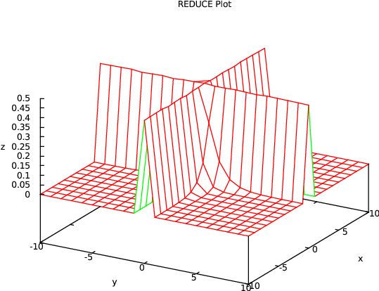
(Note the left-handed coordinate system since \(y\) is specified before \(x\) among the options; for a right-handed coordinate system specify \(x\) before \(y\).)

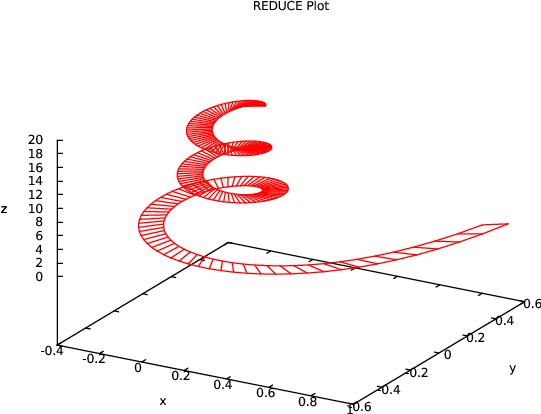
on rounded;
w:= {for j:=1 step 0.1 until 20 collect
       {1/j*sin j, 1/j*cos j, j},
     for j:=1 step 0.1 until 20 collect
       {(0.1+1/j)*sin j, (0.1+1/j)*cos j, j} }$
plot w;

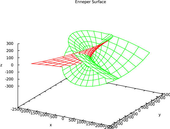
The following example is taken from: Cox, Little, O’Shea, Ideals, Varieties and Algorithms:

plot(point(3u+3u*v^2-u^3, 3v+3u^2*v-v^3, 3u^2-3v^2),
     hidden3d, title="Enneper Surface");

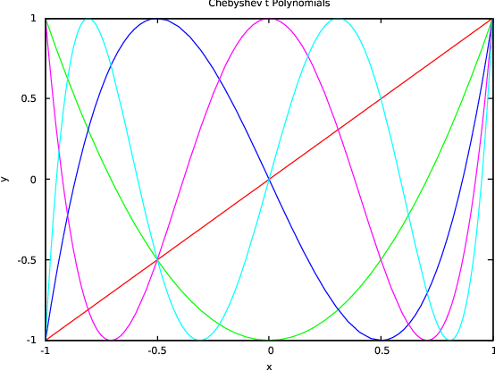
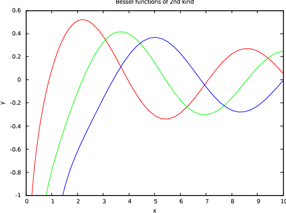
The following examples use the specfn package to draw a collection of Chebyshev T polynomials and Bessel Y functions. The special function package has to be loaded explicitely to make the operator ChebyshevT and BesselY available.

load_package specfn;
plot(chebyshevt(1,x), chebyshevt(2,x), chebyshevt(3,x),
     chebyshevt(4,x), chebyshevt(5,x),
     x=(-1 .. 1), title="Chebyshev t Polynomials");

plot(bessely(0,x), bessely(1,x), bessely(2,x),
     x=(0.1 .. 10), y=(-1 .. 1),
     title="Bessel functions of 2nd kind");

Hosted by